Inverted Pendulum
Presentation
Stabilization of an inverted pendulum is a common engineering challenge. Objective is to build a low-cost DIY1 platform to test various feedback control loop.
This document describes the hardware and the theoretical model of the pendulum. Simulation are presented with Simulink models and an LQR2 feedback control loop finally stabilizes the platform.
Video of the stabilized platform with a 4 state LQR feedback loop. The platform is completely autonomous (no user input).
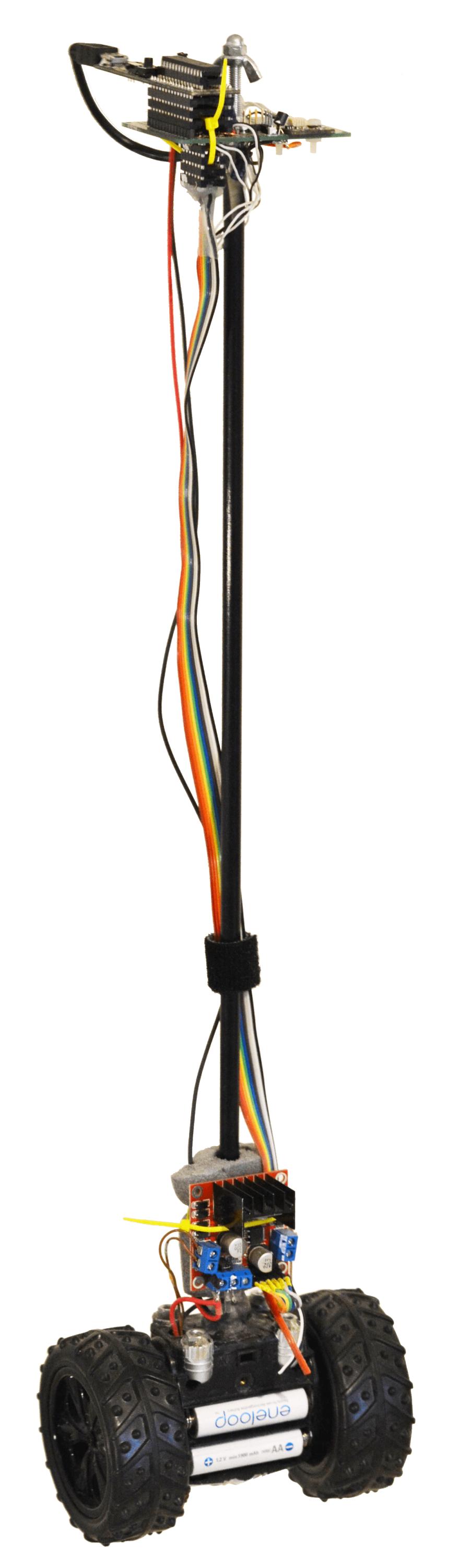
The electronic placed at the top of the pendulum composed of a dsPIC 16 bits microcontroller and an inertial sensor (accelerometers and rate gyro). The base of the pendulum is a modified RC toys comprising two wheels driven by two independent DC motor (see pictures below).
Hardware
Overview
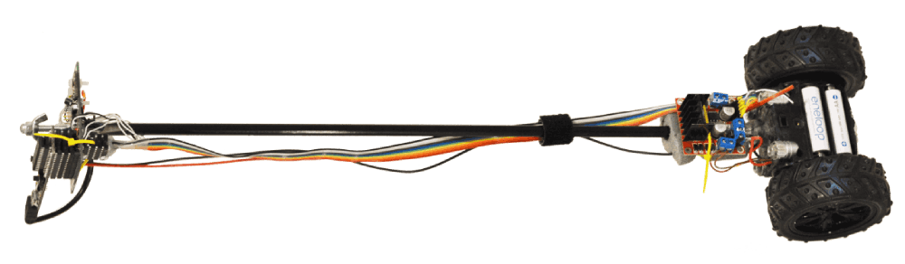
The head and the base trolley are described successively. They are separated with an $8mm$ carbon tube. The pendulum length is $0.52m$ from wheel axis to the top. Wheels diameters is $8cm$. Pendulum total weight is $200g$ comprising $111g$ for the 4 AA batteries.
Head electronics
Microcontroller
The controller is a Microstick II board equipped with a dsPIC 33EP128MC202 running at $70\ MIPS$.
It is powered through the USB connector which only provide the power supply from 4 AA batteries hold in the base.
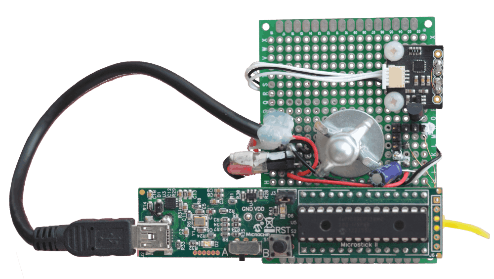
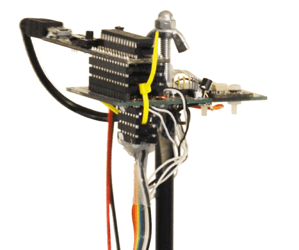
Microcontroller and sensor on top of the inverted pendulum
A prototyping board support a Microstick II board with the dsPIC 33EP128MC202. A board from Drotek endowing the Invensense ICM-20608 inertial sensor is screwed on the base board.
IMU sensor
The unique sensor used is the 6 DoF3 Invensense ICM-20608 mounted on a Drotek sensor board. It endows:
- a 3 axis Accelerometers and
- a 3 axis rate gyros.
The I2C blocks set the BUS clock at $400kHz$ and fetch the 6 sensors values every $1ms$ $(1kHz)$. The Simulink I2C blocks setting enable hot plug of the I2C sensor: The microcontroller initializes the sensor each time it is newly detected on the I2C bus.
- The accelerometer is configured with a range of $\pm 8g$ low pass filtered at $99Hz$.
- The rage gyro is configured with a range of $\pm 500 \deg/s$ low pass filtered at $250Hz$.
A Simulink IMU4 sub-system run a data fusion algorithm to reconstruct a drift-free quaternion angular position at $1kHz$ (the yaw angle drift when magnetometer is not present). The stabilization control loop uses the drift-free pitch angle.
It is possible to use other sensors like the MPU9250 or MPU6050 with either an I2C or SPI interface. The GY-91 board is a 10 DoF3 widespread board based on the 9 DoF MPU9250 (3 accelerometers, 3 magnetometers, 3 rate gyros) and has a pressure sensor.
UART interface
The PCB board provides a $3.3V$ regulator and 4 pin extra interface ( GND, +3.3v, Tx, Rx ) to connect either an UART data-logger or radio link for telemetry module or an RC receiver capable of S.BUS, Smart Port or P.Port protocol (all UART based).
Base trolley
Motors
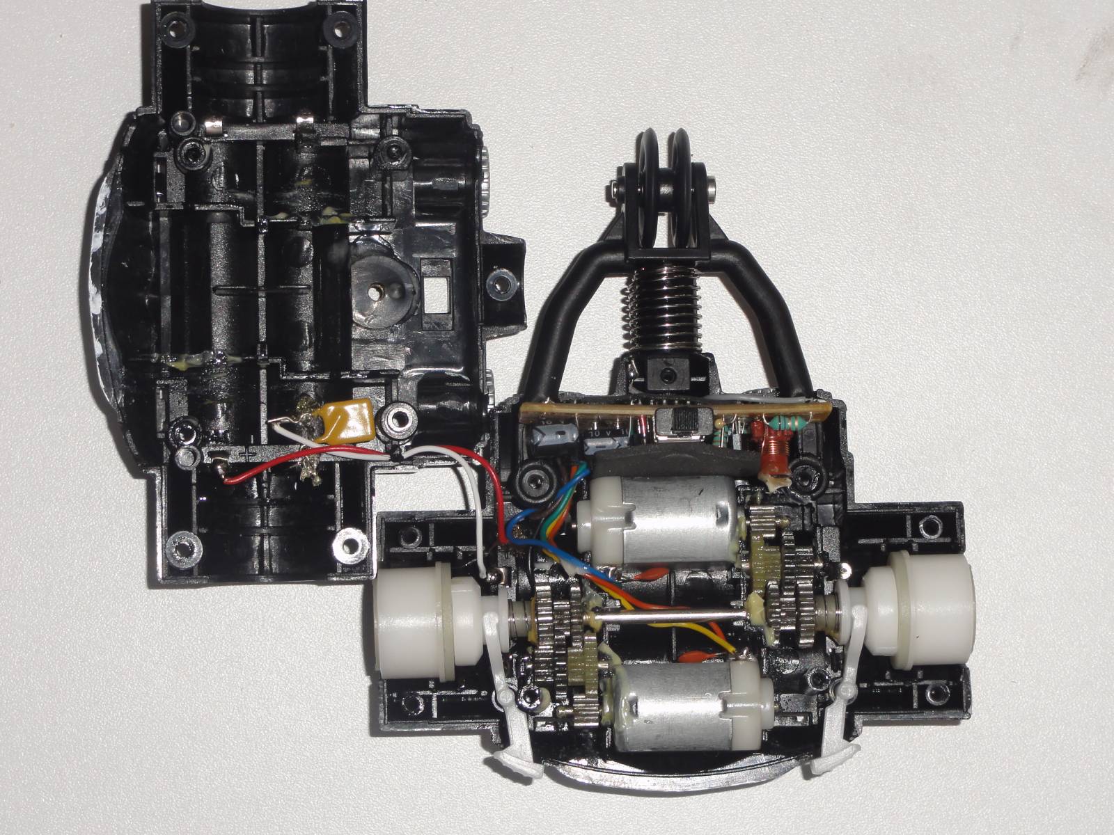
The base trolley is a low cost a 2-wheel remote control toy named flywheels. The toy is from 2012 but 2 wheeled equivalents exist.
Its electronics is removed.
Two pairs of wires power two DC motors in either direction through an L298N H bridge board module.

Power electronics
The L298N H bridge controls two DC motors. For each motor:
- Two logic signals set the 4 states: direction CW or CCW, brake, or freewheel.
- The third logic signal power the motor depending on to the state defined.
The third signal is modulated with a 100Hz square periodic signal whose duty cycle vary from 0% to 100% (PWM). It sets the torque for the motor.
The flat multicolor ribbon connects 6 logic control signals (3 for each motor) from the Microstick II dsPIC output to the of the L298N H bridge.
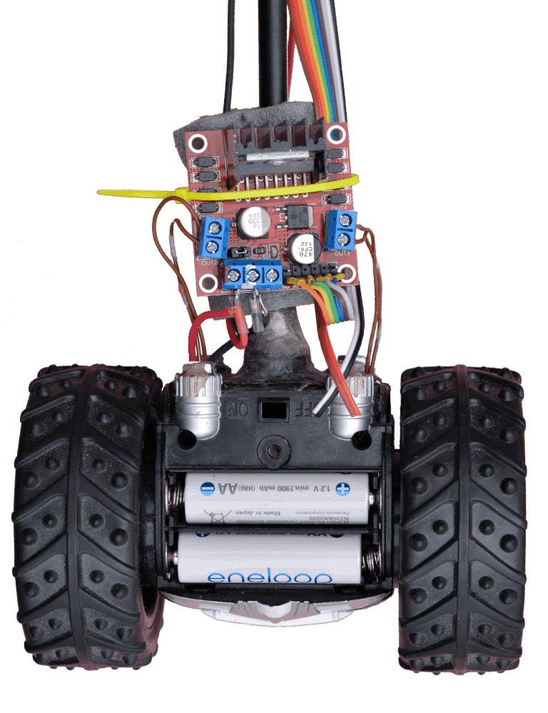
Base trolley of the inverted pendulum
A L298N H bridge (for Arduino) power board drives the two DC motors of a modified FlyWheels toy. Four AA batteries powers the pendulum.
Batteries
Four $1.2V$ AA Ni-Mh batteries are dispatched on both side of the trolley. $\approx 4.8V$ powers the motors and the electronics. The black and red wire from the trolley to the top of the pendulum powers the Microstick II electronic and sensors.
Pendulum Model
The pendulum model is composed of two intertwined sub-system:
- The pendulum*, with 1 rotation DoF3 $\theta$ angle around the wheel’s axis
- The trolley*, with 1 translation DoF3 $x$ position.
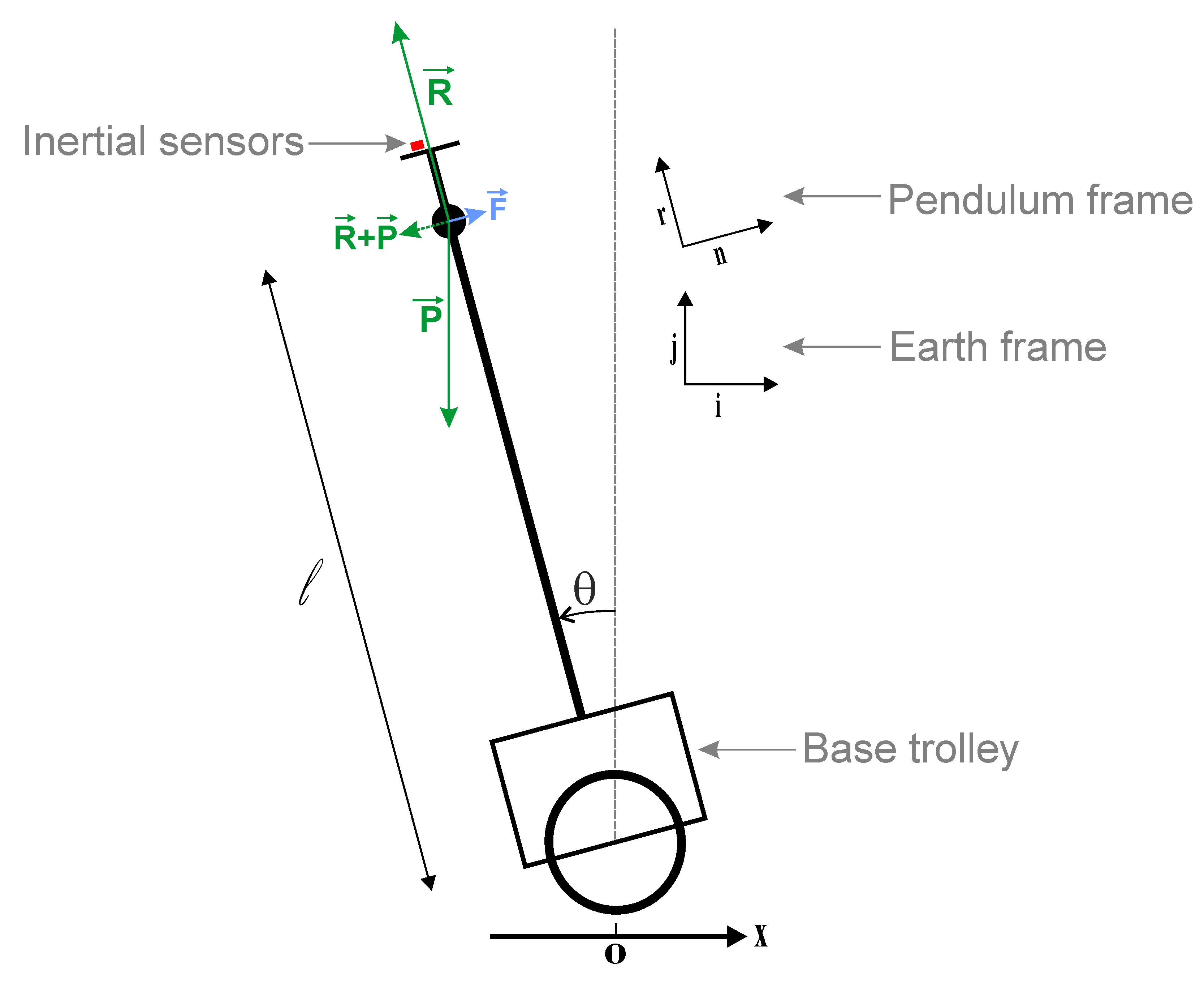
Pendulum free body diagram
$\vec{P}$ is the weight at the center of gravity. $\vec{R}$ is the reaction force from the stiff rod and the floor. $\vec{F}$ is a friction force when the pendulum is rotating. $\{ \vec{i},\vec{j} \}$ is the earth frame and $\{ \vec{r},\vec{n} \}$ is the rotating pendulum frame. The inertial sensors are placed on top of the pendulum and measure all accelerations.
Pendulum Equations
The Dynamic fundamental law applied on the pendulum: $$ \sum \vec{Force} = m.\vec{a} $$
The three forces presents are the weight $\vec{P}$, the Friction $\vec{F}$, and the Reaction $\vec{R}$ from the rod & floor:
$$ \underbrace{ -mg\vec{j} }_{\vec{P}} \ - \ \underbrace{ k \frac{\partial \vec{r}}{\partial t} }_{\vec{F}} \ + \ \underbrace{ ( mg\vec{j} . \vec{r} + \underbrace{Ctfg}_{\text{Centrifugal}} } _{\vec{R} } ) . \vec{r} = ml \frac{\partial^2\vec{ r }}{\partial t^2} $$
With $ \{ \vec{i},\vec{j} \} $ the static earth frame and $ \{ \vec{r},\vec{n} \} $ the pendulum frame (rod and normal direction). $m$ is the mass of the pendulum (without the trolley). $l$ is the length from the inter-wheel’s axis to the center of mass of the pendulum (without the trolley)
$$ \left\{ \begin{array}{rcl} \vec{i} & = & \vec{n} . cos(\theta) - \vec{r} . sin(\theta) \\\ \vec{j} & = & \vec{n} . sin(\theta) + \vec{r} . cos(\theta) \end{array} \right. $$
$$\vec{j}.\vec{r} = cos(\theta)$$
Considering the rotation $\theta$, the first and second time derivative of $\vec{r}$ are:
$$ \begin{array}{rcl} \frac{\partial \vec{r}}{\partial t} & = & - \dot{\theta} \vec{n} \\\ \frac{\partial^2\vec{ r }}{\partial t^2} & = & - \frac{\partial }{\partial t} \left( \dot{\theta} \vec{n} \right) \\\ & = & - \ddot{\theta} \vec{n} - \dot{\theta}^2 \vec{r} \end{array} $$
The projection of the forces equation in the pendulum frame $ \{ \vec{r},\vec{n} \} $ is:
$$
\left\{ \begin{array}{rcl}
\left( ml\dot{\theta}^2 + Ctfg \right) \vec{r} = \vec{0} \\\
\left( l \ddot{\theta} + \frac{k}{m}\dot{\theta} - g . sin(\theta) \right) \vec{n} = \vec{0}
\end{array} \right.
$$
The first equation for the $\vec{r}$ axis shows internal forces which cancel each other: the weight $\vec{P} = -mg\vec{j}$ which is compensated on the $\vec{r}$ axis by the term $mg\vec{j}.\vec{r}$ from the reaction force which will also compensate for the Centrifugal force $ml\dot{\theta}^2$.
The second differential equation on the $\vec{n}$ axis allows to solve for the evolution of the angle $\theta$. It can be made linear with $sin(\theta) \approx \theta$ when the pendulum is up near $0$, or with $sin(\theta) \approx - (\theta - \pi)$ when the pendulum is down near $\pi$.
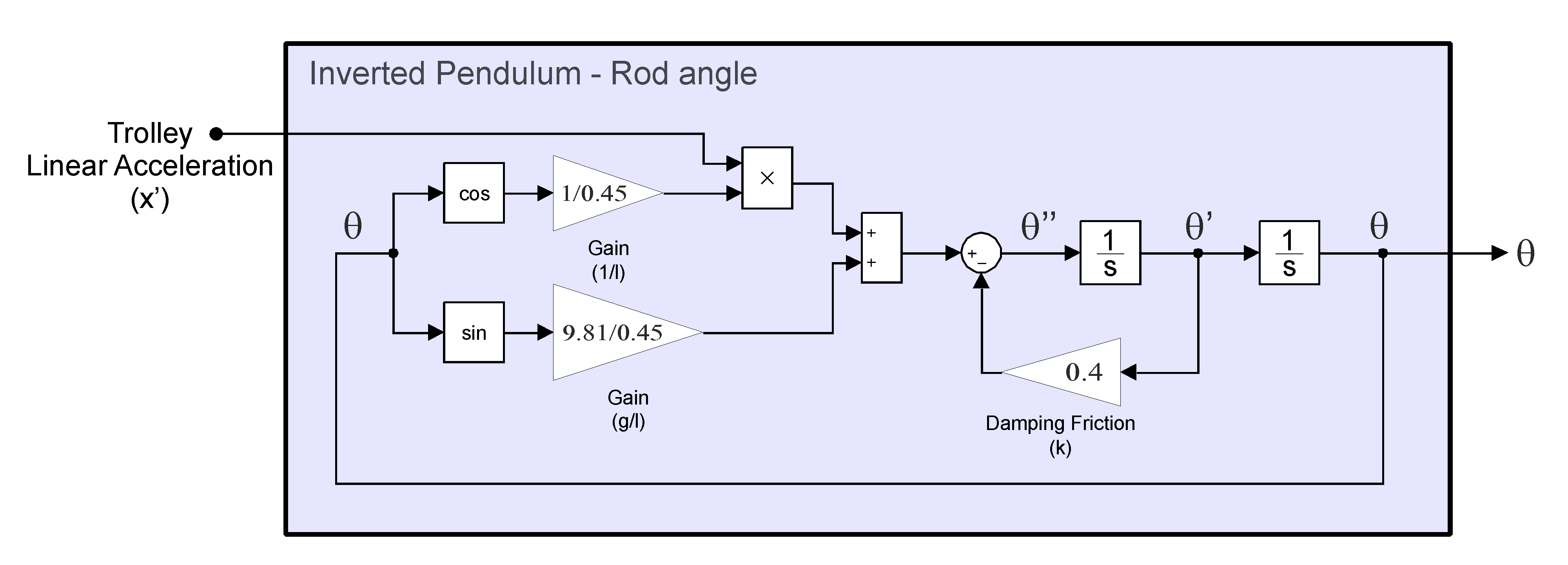
Pendulum model for rod rotation
non-linear model of the $\theta$ angle evolution derived from the forces projected on the normal $\vec{n}$ axis of the rod. The trolley linear acceleration input is added.
The linear approximation for $\theta$ in the laplace domain is a $2^{nd}$ order system: $$ \theta(s) \left ( \frac{1}{w_n^2}s^2 + \frac{2 \zeta}{w_n}s \pm 1 \right ) = 0 $$
The pendulum transfer function $F_p = \frac{\theta(s)}{E(s)}$ with a null input $E(s) = 1$ $$ F_p(s) = \frac{1}{ \frac{1}{w_n^2}s^2 + \frac{2 \zeta}{w_n}s \pm 1 } $$
This transfer function is characterized when the pendulum is down by its natural frequency $w_n = \sqrt{ \frac{g}{l} } $, and a damping factor $\zeta$.
Pendul identification
The parameter $l$ could be estimated from the platform mechanical but the damping parameter $\zeta$ (or frictions coefficient $k$) could not be estimated easily from the platform.
The simulation model is satisfactory when the calculation it performs make realistic prediction. Experimental measurement is a good method to refine a model and tune its parameters. In our case, the parameters $l$ and $\zeta$ (or $k$) are identified from the experiment explained below.
Experimental logs
The pendulum is placed on a track (two chairs back to back) to be able to make a complete rotation. Motor are off and the pendulum is released up-side with in the unstable condition ($\theta = -18°$ , $\dot \theta = 0$).
It oscillates until the damping friction ($\zeta$) stops the free oscillations.
The $1kHz$ sampled rate gyro and accelerometers values are recorded onboard an openlager board connected on the dsPIC UART interface.
Simulation from logs
The measured inertial sensors are then re-used as data source in a Simulink model. $\theta$ angle is reconstructed using an IMU complementary filter algorithm implemented in the quaternion angle representation.
The pendulum model is initialized with the experimentation initial condition ($\theta = -18°$ , $\dot \theta = 0$). Trolley linear acceleration input is null. Parameters $l$ and $k$ are iteratively tuned until the model $\hat{\theta}$ angle fit with the measured oscillation $\theta$.
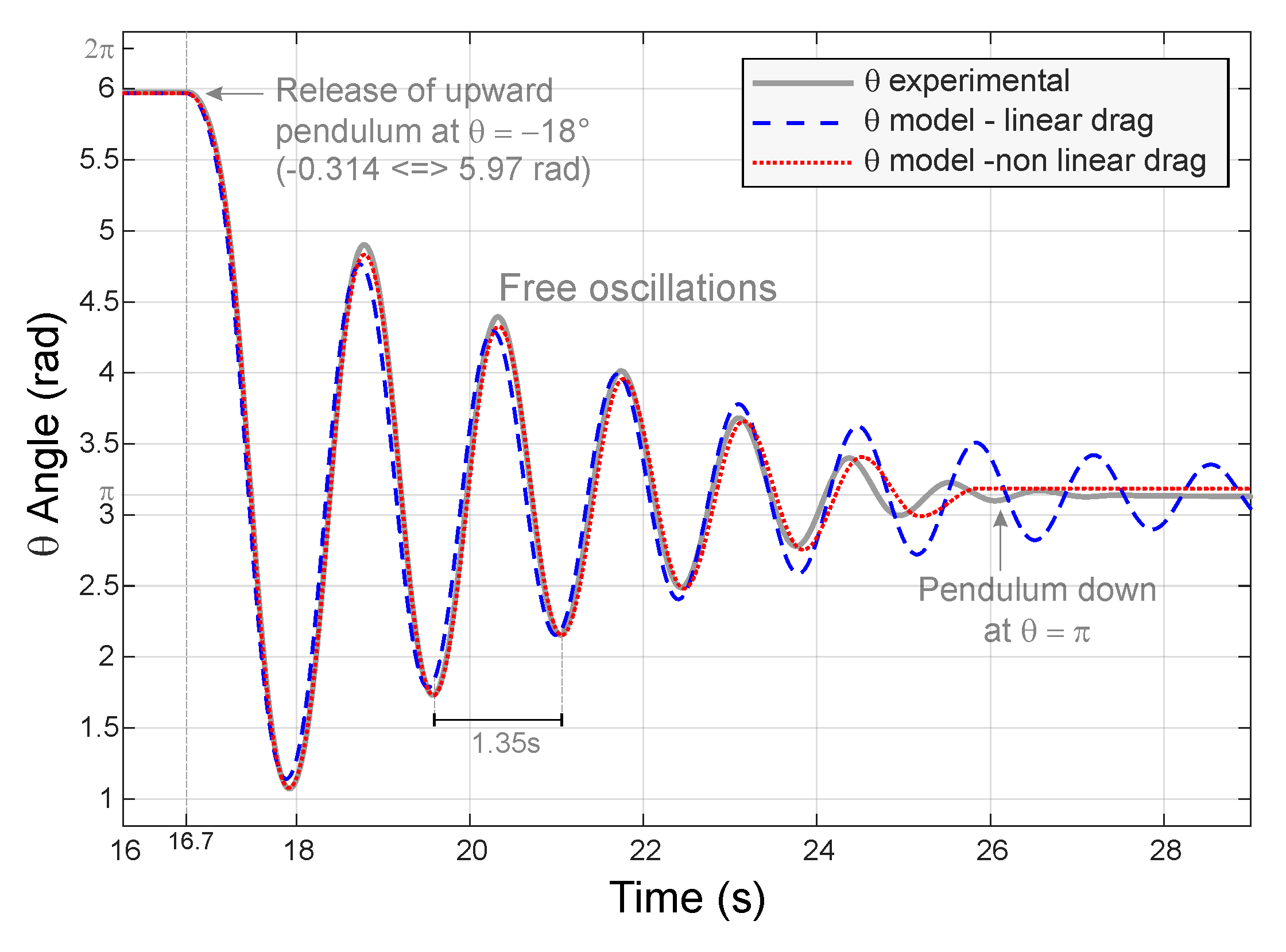
Identification - experimental $\theta$ angle reconstructed from inertial sensors (wide grey curve) vs pendulum model (read and blue dashed curves)
$\theta$ angle from free oscillation experiment is compared against two pendulum models. The pendulum is released at time $16.7s$ upside ($18°$) and let free to oscillate. The grey curve is the experimental angle reference reconstructed from inertial sensors measurements. The blue dashed curve is a pendulum model using a linear damping with $k = 0.4$. The red doted curve use a nonlinear damping with the nonlinear term -1.1*$sign(\dot{\theta})$ added to the linear damping with $k = 0.17$.
| Pendulum Parameters | Identified Value |
|---|---|
| $l$ | $0.45 m$ |
| $k$ | $0.4$ |
| $w_n = \sqrt{\frac{g}{l}}$ | $4.67\ rad.s^{-1}$ ( $0.74 Hz$ or $1.35s$ period ) |
| ⬆ Identified pendulum parameters |
Validation and IMU improvement
Parameters $l$ and $k$ can be further validated using the force equation and the estimated pendulum angle $\theta$.
The IMU input measurements is composed of the rate gyro and the accelerometers data. Magnetometers is not used in this pendulum example. The IMU input also require the predicted acceleration vector (resp magnetometer is used). The IMU output the sensor orientation and provides the gravity vector prediction as seen in the sensor estimated attitude (i.e. quaternion angle).
Comparing the gravity vector predicted with the accelerometer’s measurement do not match because the sensor measures both the gravity plus the dynamic acceleration induced by the pendulum movements.
Considering the pendulum principal movement rotation $\theta$, the equations of forces applied on the pendulum derive from $\hat \theta$ a prediction for the dynamic acceleration. The good match between the predicted acceleration and the experimental measurement confirm somehow the correctness of parameters $l$ and $k$ involved in these calculations.
The updated acceleration comprising both a static and dynamic part is fed into the IMU algorithm improving the IMU correction of the rate gyro integration drift even when the pendulum is not static.
Trolley Model
Trolley Equations
The translational movement of the trolley is modeled as a $1^{st}$ order system characterized by its time constant $\tau$. This dynamic includes the motor dynamics when it is loaded with the trolley considering the pendulum as vertical.
The model considers as negligible the effect of the pendulum forces (translational and rotational) applied on the trolley.
$$ x(s) = \frac{1}{\tau s + 1} $$
Trolley Identification
| Trolley Parameter | Estimated Value |
|---|---|
| $\tau$ | $0.3s$ |
The trolley does not have any sensors. No encoder or current sensor are used to control the two motors. The parameters $\tau$ is “guessed” in a first step. In a second step, a $2^{nd}$ inertial sensor board is temporary glued in the middle of the wheel diameter to as the inertial sensor is in the wheel rotation axe. An identification can be computed from the motor set-point and the wheel movements while the pendulum was actively controlled up by a first feedback loop.
Still the pendulum model including the trolley is simulated with its feedback loop controller and results are compared against recorded data of the real system running the same feedback loop controller. The simulated pendulum states are re-initialized periodically ($\approx 2s$) with the real pendulum states as the model would diverge otherwise due to perturbations not modeled and model discrepancies. Correctness of the model can be checked between these periodic re-initializations.
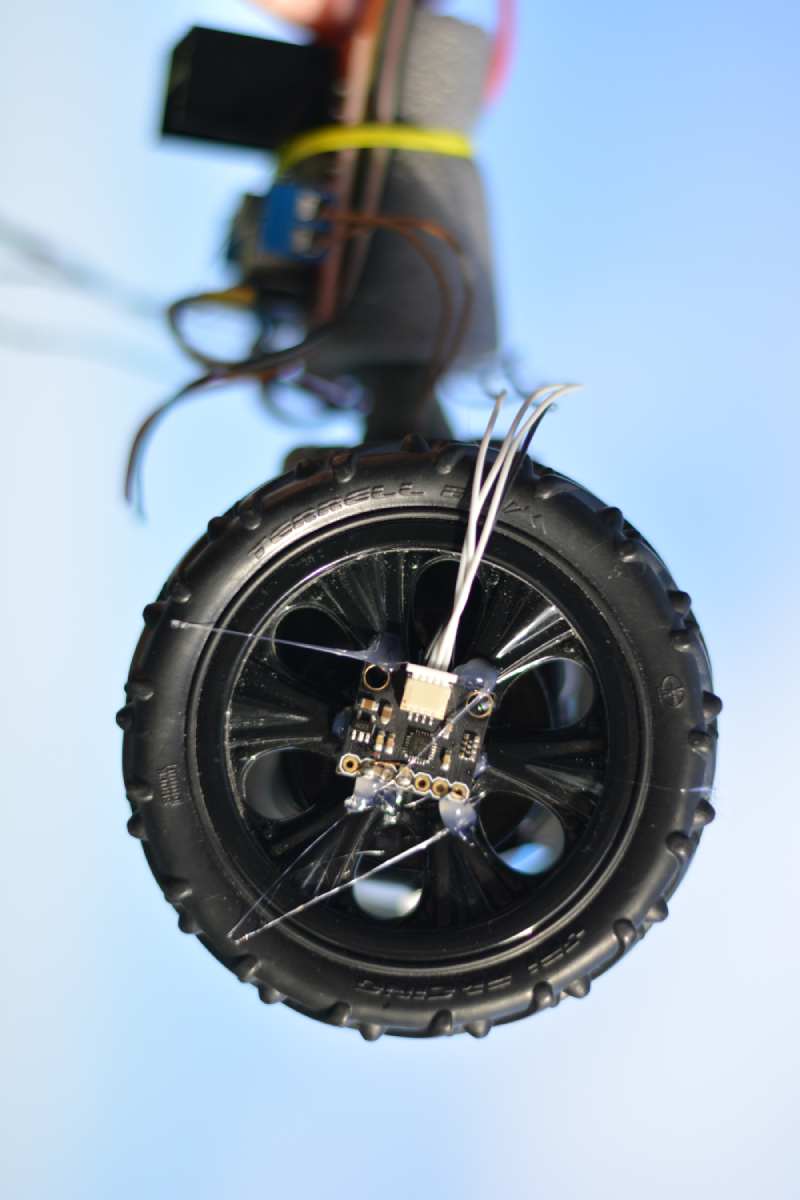
Identification of trolley in real inverted pendulum condition.
The angular speed rate of the wheel is measured with one rate gyro form one added GY-91 sensor board. The GY-91 board is hot glued on one pendulum wheel. The pendulum is stabilized with a controller using an estimated trolley model. Four wires from the GY-91 to the microcontroller power the sensor and retrieve sensor data through the I2C bus (2 wires).
Controller
Stabilization overview: The microcontroller computes the angle of the pendulum from the inertial sensor measurements (accelerometers and rate gyro). A feedback loop stabilizes the pendulum up right while maintaining the pendulum position still. The pendulum translation is estimated through an internal dynamic model of the trolley stimulated with a copy of the DC motor command. The pendulum slow translations reflect the drift of the internal estimation of the displacement.
Linearized model
LQR feedback controller
Video of the inverted Pendulum when it encounters a wall:
Another way to stabilize a pendulum with an electric seesaw (video).