Miniature airspeed sensor for RC plane and UAVs.
A Pitot static (Prandtl) airspeed sensor embedded in an RC plane: Parts, Electronic and Performances.
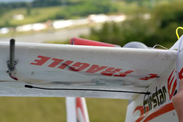 Carbon Pitot-tube attached to the wing with a magnet.
Table of Contents
Pitot tube principle
A Pitot-Darcy probe is an airspeed sensor commonly used in aviation. It consists of a tube pointing in the forward direction. When the sensor moves forward a stop pressure $P_t$ is added at its tip. The differential pressure $P_{diff}$ is measured between the tip of the tube $P_t$ and the static pressure $P_s$. One variant named from its inventor Prandtl tube has static air ports directly on the side of the tube.
The pressure added at tube tip is the square of the airspeed : $P_t = P_s + \frac{1}{2}\rho v^2$ where $ P_t $ and $P_s$ are measured in Pascal unit (Pa). $\rho$ is the air density constant typically in $[1.14 \ 1.34]$ depending on temperature & altitude. $v$ is the airspeed in $m.s^{-1}$. The differential pressure measured is $P_{diff} = P_t - P_s = \frac{1}{2}\rho v^2$
Pitot-Prandtl tube
Prandtl tube is one version of a Pitot probe where an inner tube is placed in the center of an outer tube. Space between the two tubes is filled-in on few mm near the tip with an epoxy adhesive (Araldite or equivalent). The side of the outer tube is drilled to sense the static pressure. At the bottom, the inner tube which is longer act as a connector for the dynamic pressure sensor and third short tube is added to create a connector to the static pressure area which lies in the empty space between the two tube.
The static pressure holes must be drilled at a minimum distance from the tube tip where airflow perturbations are reduced. A distance 4 times the diameter (d=4mm)of the outer tube is retains here (16mm). Four 1mm holes were drilled with a Dremel hand tool. The three tubes are presented on the figure below.
First test was done using brass tubes. Inner tube width is 2/1mm (outside/inside) and outer tube is 4/3mm.
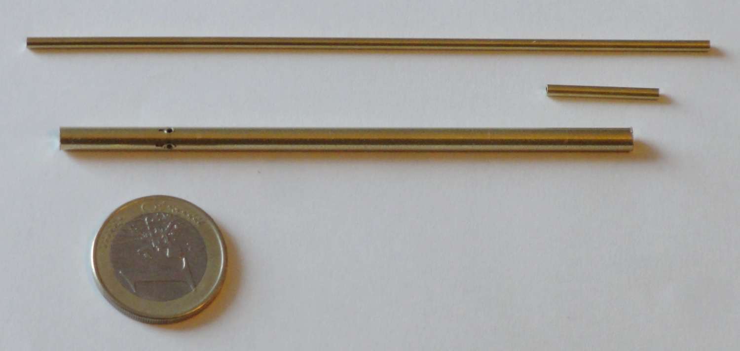
Brass inner and outer tubes of the Pitot tube.
Tube alfer from Leroy Merlin. Inner tube is 2mm/1mm. Outer tube is 4mm/3mm. Outer tube length is m=86mm. Four 1mm holes are drilled at l=16mm from the tip.
References:
- report WIND-TUNNEL INVESTIGATION OF ‘A NUMBER OF TOTAL-PRESSURE TUBES AT HIGH ANGLES OF ATTACK SUBSONIC, TRANSONIC, AND SUPERSONIC SPEEDS’ by W.Gracey on the impact of the various shape on the measurement.
- report (french) from ANSTJ with general information on Pitot sensor.
- website (French) from Rémi Bourgin with experimental Pitot tube for RC plane
Electronics
Sensitivity requirements and Pressure sensor
The differential pressure measured vary with the square of the speed. RC plane speed can be quite low. Challenge is to be sensitive enough to obtain good measurement even in the low speed range of few meters per seconds.
The MP3V5004dp from NXP is a sensitive differential pressure sensor. Its differential measurement range goes from 0 to 3.92 kPa. The analog output is ratio-metric and swing from 0.6V to 3V ($\Delta V =2.4V$). For reference, 1 kPa is approximately the pressure of 10cm of water.
We are interested in speed range varying from $0$ to $25 m.s^{-1}$ ($90km/h$) which correspond to a maximum differential pressure of 3.75 cm of water, or 0.375 kPa. The MP3V5004DP sensor is used in 10% of its nominal range.
Table below provide theoretical differential pressure expected for various speed using $P_{diff} = \frac{1}{2}\rho v^2$ with $\rho=1.15$.
| v (m/s) | v (Km/h) | $P_{diff}$ (Pa) | ~ $H_2O$ (cm) | MP3V5004dp & MCP3428 (0.2041Pa / LSB1) |
|---|---|---|---|---|
| 1 | 3.6 | 0.6 | 0.006 | 3 |
| 2 | 7.2 | 2.4 | 0.024 | 12 |
| 4 | 14.4 | 9.6 | 0.096 | 47 |
| 7 | 25.2 | 29.4 | 0.294 | 144 |
| 10 | 36 | 60 | 0.6 | 294 |
| 15 | 54 | 135 | 1.3 | 661 |
| 20 | 72 | 240 | 2.4 | 1176 |
| 25 | 90 | 375 | 3.75 | 1837 |
| 30 | 108 | 540 | 5.4 | 2646 |
| 40 | 144 | 960 | 9.6 | 4704 (4095 sat) |
Signal conditioning and conversion
The pressure sensor electronics is placed in the wing close (~10cm) to the Pitot tube. The analog to digital conversion is integrated in the sensor board. The MCP3428 from Microchip is a high resolution sigma-delta converter with a programmable gain factor from 1 to 8. It has a digital I2C bus interface and its I2C address can be selected. Similar DAC to consider are MCP342x, the newer MCP346x family or the MCP356x providing increased accuracy and higher sampling rate but its package is smaller thus more difficult to handle for a DIY project.
The MP3V5004dp output analog signal is connected to the MCP3428 Sigma-Delta ADC through a first order RC low pass filter with a cut off frequency at $28Hz$ ($R=5.6 kOhm$,$C=1\mu F$). The 2nd differential input is connected on a voltage divisor to obtain 1V from the 3.3V reference (480 & 1kOhms). $10\mu F$ decoupling capacitor are used on power supply. The I2C bus wires are pulled up with 10kOhm and are connected to a 10pf capacitor protecting from glitches.
The MCP3428 Sigma-Delta ADC is configured for
- 12 bits
- x8 Gain
- 240 Samples Per Seconds (SPS)
The resulting resolution is provided from:
- (1) MP3V5004dp Analog output sensitivity is 1633 Pa/V
- (2) MCP3428 12 bits with a gain of 8 : 0.125mV/LSB1
With (1) and (2), we obtain a resolution of $1633 * 0.125e^{-3} $ = 0.2041 Pa / LSB1
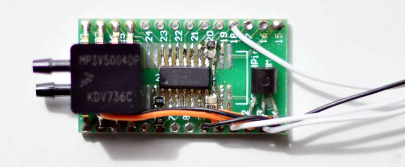
Pressure sensor and electronics mounted on a DIP adapter board.
Differential pressure sensor (MP3V5004dp) with Analog to Digital converter integrating a differential amplifier (MCP3428). The MCP3428 communicate with the microcontroller through an I2C BUS. A MCP1700 3.3V voltage regulator adapt and filter out the 5V input voltage.
Sensor static tests
A 90 minutes lasting measurement is performed indoor without movements. Sensor output were logged at 100Hz. The figure below shows a slow drift (correlated with temperature or battery decay ? TBD). The sensor standard deviation measured on the overall measurement is 0.54 Pa (including the drift).
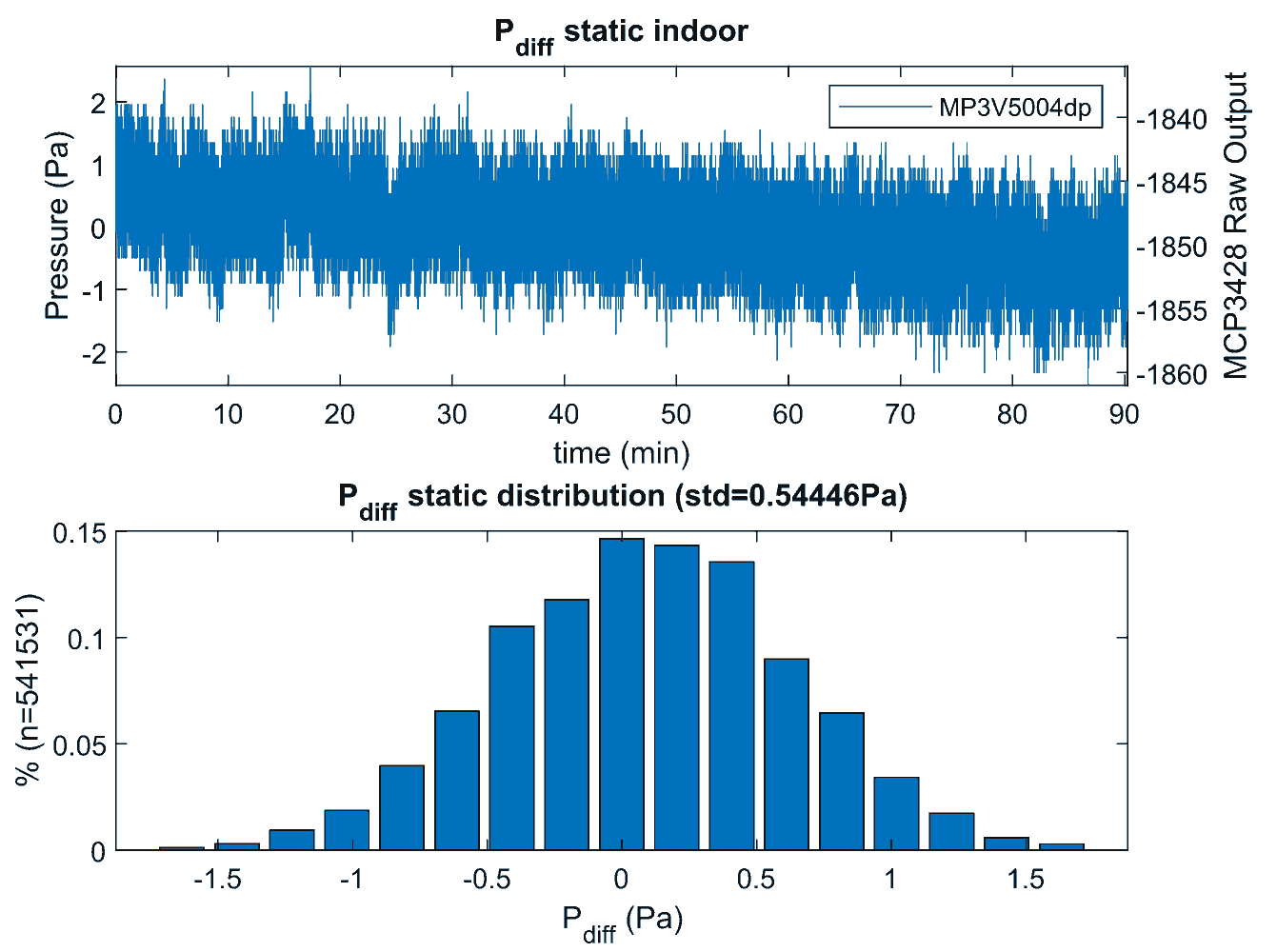
Experimental pitot-tube static characteristic with the MP3V5004dp differential pressure sensor
90 minutes lasting static measurement indoor shows a slow drift and a standard deviation of 0.54 Pa. Resolution is 0.2041 Pa / LSB
possible noise/offset sources
The sensor is sensitive to its own orientation. Flipping the sensor up-side down creates an negative offset of 12.5mV (100 LSB1 with the analog to digital circuit setting).
MCP5398 and MP3V5004dp are both powered with 3.3V. A linear voltage regulator (MCP 1700) filter-out the 5V sensor board input to 3.3V. The analog signal remains however sensitive to fluctuation on the 5v input. Particular attention should be taken with telemetry which pollute power supply if they do not have their dedicated regulator. Also the electromagnetic burst from telemetry module might pollute the overall electronic including the ground; A periodic burst correlated with MAVLink packets sent was noticed on pitot output (20 to 300 LSB, nothing noticed on IMU sensors) caused by a 3DR telemetry module when its antenna is placed too close to non protected electronics part. Problem solved by moving the antenna away and reducing the Tx emitting power.
Flight setup
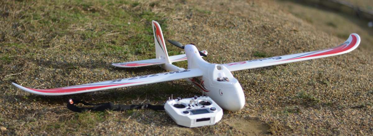
The sensor is mounted on the wing of a FirStar 1600 RC plane.
A 2mm flexible tube, originally for protecting fish lines, connect the sensor to the Pitot tube.
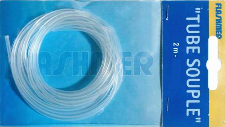
Flashmer – flexible Tube 2mm. Image from Decathlon (france).
Fishing Tube used to connect the differential pressure MP3V5004dp sensor to Pitot tube.
One magnet is glued on the Pitot tube. A 2nd magnet integrated in the wing allows to fix the Pitot tube. Both magnet are in contact. The tube stays firmly in place during flights and ejects in case of hard landing reducing damages. It is a flexible solution for testing other Pitot tube design ; It’s also practical for storage and transportation.

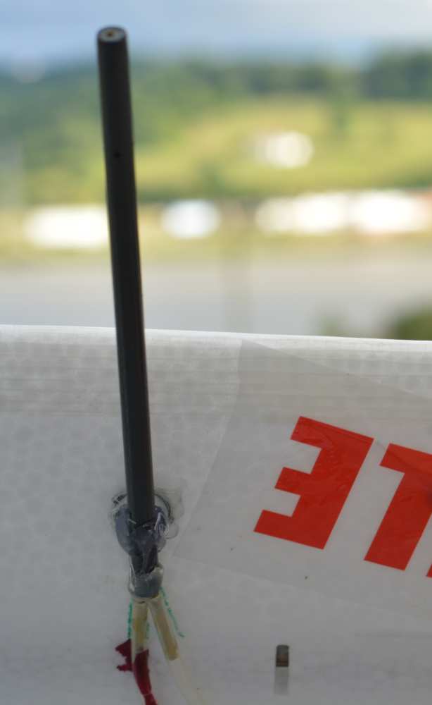
Carbon-Brass light Pitot tube sensor attached to the wing with a magnet.
Outer tube is a 5/3mm carbon tube. Inner tube is a brass 2mm/1mm tube.
Experimental results
The MCP3428 samples $P_{diff}$ at 250Hz during flights. $V_{Pitot}=\sqrt{\frac{2}{\rho}*P_{diff}}$ with $\rho = 1.15$.
No calibration were required. Sensor theoretical output scaling were used with the formula to compute the speed from the pressure. $\rho$ value was tune from a default value 1.2 to 1.16 which minimized the mean error however the improvement was not a big deal. The only value to adjust is the raw pressure measurement offset (zero). The zero value for the sensor used is -1800.
Matlab script converting 250Hz raw MCP3428 to Pressure (Pa) and Speed (m/s):
% Pitot Calibration. P_pitot is a vector with raw MCP3428 output read from I2C bus.
P_pitot_cal =  0.2041* (double(P_pitot) + 1800);	% to Pa unit

% Compute Speed (m/s) from diff pressure (in Pa).
V_pitot = sqrt(max(0,(2/1.15) * P_pitot_cal));
Comparison with GPS ground speed
In calm condition, the ground speed $V_{GPS}$ and airspeed $V_{Pitot}$ are equal.
In windy condition, wind average direction and strength are estimated combining $V_{GPS}$, $V_{Pitot}$ and the plane yaw $\Theta_{heading}$ direction (using GPS COG2). This wind estimation is described below.
The airplane ground speed (GPS) is estimated with the difference of the airspeed (Pitot) with the projected wind to the aircraft forward direction:
$V_{GPS} \approx V_{Pitot} - V_{wind}*cos(\Theta_{heading} + \Theta_{wind}) $
The figure below presents the airspeed in blue. The reconstructed ground speed (black) matches accurately with the GPS velocity (red) which prove the correctness of the airspeed measurement as well as the wind strength and direction. The onshore wind is laminar with limited turbulences. The airspeed measurement presents a high sensitivity even at low speed.
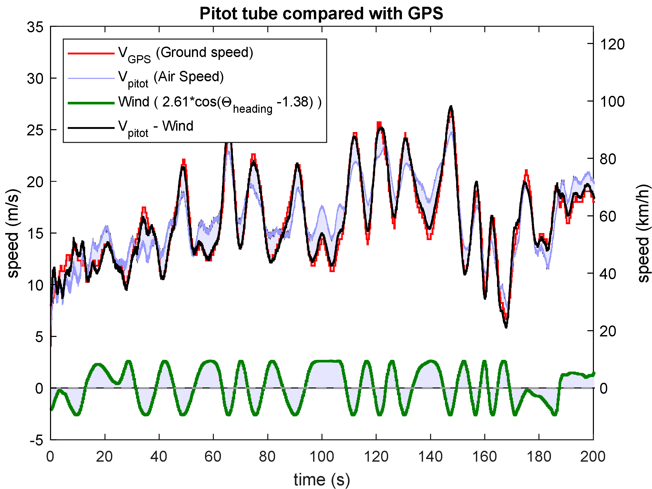
Experimental measurement comparing GPS ground speed with pitot-tube airspeed on 200s of a Firstar 1600 RC plane flight. Match between the GPS ground speed and the pitot tube subtracted from the estimated wind.
GPS Speed over ground (red). Pitot airspeed (blue) computed with $\rho=1.15$. Reconstructed up-front wind (green). Pitot airspeed minus wind estimated (black) where $V_pitot$ is averaged and under-sampled by a factor 5 reducing its sampling rate from 250Hz to 50Hz. Up-front wind is estimated from the GPS COG angle ($\approx \theta_{heading}$), and the estimated wind strength ($V_{wind}= 2.5 m/s$) and direction ($\theta_{wind} = 101°$).
More figures in online presentation.
The GPS update rate is 10Hz. It is sampled at 50Hz to minimize delay. The pitot-tube sensor update rate is 260Hs but it is sampled at 250Hz.
The error is defined with $error = V_{gps} - \left( V_{Pitot} - V_{wind}*cos(\Theta_{heading} + \Theta_{wind}) \right) $. For the 200s of the flight shown on the figure, the error measured is:
| error | m/s | km/h |
|---|---|---|
| mean | 0.017 | 0.06 |
| standard deviation | 0.74 | 2.6 |
RMS error is relatively low regarding the measured speed value. Part of the error is also due to wind gust and GPS limited accuracy particularly at estimating fast change of vertical speed.
Wind estimation
Wind model considered is constant and characterized by
- its constant direction $\Theta_{wind}$
- its constant strength $V_{wind}$
Wind => $V_{Pitot} - V_{gps}$
The curve below shows the difference between the Ground speed (GPS) with the airspeed (Pitot) in function of the plane flight direction. This error (blue dashed points) fit with a sine wave. This sine wave is the speed offset added for each plane direction in $[0 \ 2\pi]$ by a wind with a constant strength and direction. Sine wave amplitude and phase is the wind strength and direction.
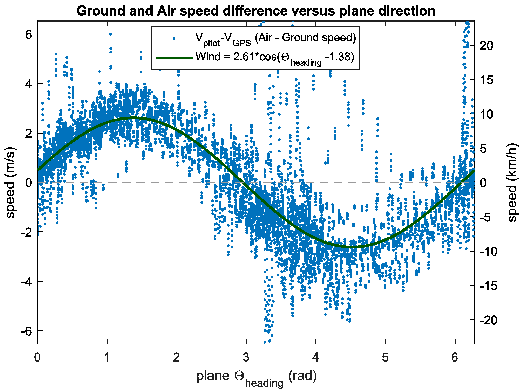
Experimental result presenting GPS ground speed and Pitot airspeed difference in function of the plane direction of 450s flight of the RC Firstar 1600 plane.
Blue dots are speed difference between GPS and Pitot. The continuous green curve is the wind sine wave projection on the $\Theta_{heading}$ plane direction. Sine phase is wind direction ($(\pi-1.37*\frac{180}{\pi})=101°$, from East to West) and sine amplitude is wind strength (2.56m/s). Pitot values are averaged and under-sample by a factor 5.
This wind estimation is used to compensate the airspeed when comparing the GPS ground speed $V_{gps}$ with the Pitot airspeed $V_{Pitot}$ above.
Script
Matlab script to estimate wind off-line:
% V_gps and V_pitot are two vector with all data measured.
% V_pitot was under-sampled (averaging) by a factor 5 to fit the 50Hz log from the GPS.
% GPS chip update frequency is 10Hz, but it is logged at 50Hz.

V_err = V_pitot -  V_gps;    % Ground and Airspeed difference (i.e. wind)

M = [cos(COG); sin(COG) ]'; % COG is the direction (Theta in rad) vector data measured from the GPS
y = V_err';
x = M\y;    % Solve wind strength and direction using linear algebra (MMSE)

Theta_Wind = -atan2(x(2),x(1));  % Wind (go to) direction. Azimuth direction is opposite to trigo
V_Wind = sqrt(sum(x(1:2).^2));  % Wind strength (m/s)

plot(COG,V_err','.'); hold on; % plot Error blue dots
plot([0:.01:(2*pi)],V_Wind*(cos([0:.01:(2*pi)]+ Theta_Wind)),'-k','linewidth',3); % plot wind
Discussion
Using the GPS COG2 field is not exactly the plane yaw direction $\Theta_{heading}$ but the plane flight direction. Thus the COG is a biased plane yaw $\Theta_{heading}$ direction. It would be best to use plane orientation from the IMU sensor. It is not done here to reduce the number of sensors for this demonstration. The COG bias is small enough if we assume the wind speed to be small compared to the airplane airspeed. It might be possible with a more sophisticated script to compensate this bias.
W. Premerlani propose a wind estimation using exclusively GPS data. Tests with this GPS dataset was not conclusive while trying to use all GPS sample while the platform direction is modified (i.e. COG derivative is above a given threshold). GPS dynamic seems too slow to provide robust results.
Other flight data
Plane was equipped with two GPS:
- one uBlox M8N GPS and
- one MTK3339.
The uBlox trace presented on the map below is better than the MTK trace. The uBlox chip was used exclusively for the curves above. The MTK trace can be shown on the map (top left icon). The KML file can be opened with Google Earth which provide a 3D view of the trace showing the height of the plane.
Lubin Kerhuel
Engineer, PhD
Interested in signal processing and control theory. 10 years experience with rapid control prototyping.